Chapter 5 Factor Models

5.1 Introduction

Analysis of structural VARs may lead to results that contradict theory and intuition on how the economy works. One such example is the ‘price puzzle’, i.e. tightening monetary policy appears to induce inflation whereas in reality the central bank reacts to rising inflation with a tighter monetary policy. () suggested that central bankers look at many other variables when deciding on their monetary policy stance. Yet, adding more variables does have its problems:

Number of parameters to estimate increases fast with the number of variables.
Many variables convey similar information (examples). Thus, to avoid collinearity problems, we have to pick a subset of available variables but we don’t know which ones we have to pick.
How do we interpret the results?

One popular method is to reduce the dimension of the problem, i.e. we approximate a large number of variables with a smaller set of latent variables or factors and hence we have to estimate a smaller number of parameters. A downside of this approach is that interpretation of factors is difficult.

We discuss two ways of estimating dynamic factor models. The 2-step approach and the state-space approach. In the 2-step approach we start with the estimation of the factor structure using a principal-components approach and in the second step we estimate the dynamic model. The state-space approach treats the factors as latent variables and is estimated using a Kalman-Filter.

Our discussion starts with estimating principal components. Not only is it the first step in our 2-step approach but we can also discuss issues such as non-uniqueness of principal components and the solution to these problems.

5.2 Principal Components

5.2.1 The Setup

Let \(Y\) be a \(n\times p\)-data matrix with entries \(Y_i=(y_1,...,y_p)\) and \(i=1,...,n\). The goal is to minimize the following least-squares equation \[\begin{equation} ||Y-Yv^\intercal v||^2 \end{equation}\] such that \(v^\intercal v=1\). The \(v\) are called the standardized linear combinations. An equivalent formulation is to maximize \[\begin{equation} ||Yv^\intercal v||^2=v^\intercal S v \end{equation}\] such that \(v^\intercal v=1\) and \(S=Y^\intercal Y\).

But how do we find these standardized linear combinations \(v\)s? For illustration we focus on maximizing \(v^\intercal S v\) in the one-dimensional case. Given the maximization problem and the constraint we can write it as follows

\[\begin{equation} \frac{d}{dv}\left(v^\intercal S v-\lambda(1-v^\intercal v)\right)=0. \end{equation}\]

This results in the following first-order condition:

\[\begin{equation} Sv=\lambda v \end{equation}\] Hence the points at which \(v^\intercal S v\) is maximized are the unit eigenvectors of \(S\).

With a fixed number of principal components we can turn to the question how much variation of the original data \(Y\) is explained by the principal components.

An important question is how many principal components we do need.

5.2.2 Examples

We now turn our attention to two examples to explain the use of principal components. The first example is from finance and is about the question how do we approximate the yield curve.

# Load libraries
library(YieldCurve)
library(ggfortify)
data(ECBYieldCurve)

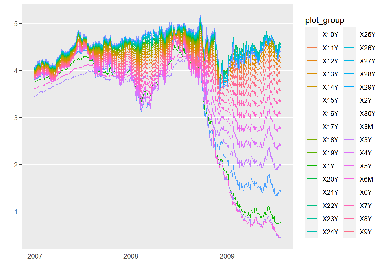
First, we plot the yield curve

autoplot(ECBYieldCurve,facets = F)

Until late 2008 the spread between short-term yields and long-term yields was relatively small. This spread widened in late 2008 and coincides with the Bankruptcy of Lehman brothers and the peak of the great financial crisis.

# Get covariance matrix
v1 <- var(scale(ECBYieldCurve))

#

As it turns out, 99% of the variation in yield curves can be explained by 3 factor.